- Tue 27 November 2018
- datascience
- #multiple regression, #XGBoost, #data cleaning
Today, I'll show my entire process for my submission to the Kaggle competition for predicting house prices.
House Prices: Advanced Regression Techniques
https://www.kaggle.com/c/house-prices-advanced-regression-techniques

Competition Description
Ask a home buyer to describe their dream house, and they probably won't begin with the height of the basement ceiling or the proximity to an east-west railroad. But this playground competition's dataset proves that much more influences price negotiations than the number of bedrooms or a white-picket fence.
With 79 explanatory variables describing (almost) every aspect of residential homes in Ames, Iowa, this competition challenges you to predict the final price of each home.
Goal
It is your job to predict the sales price for each house. For each Id in the test set, you must predict the value of the SalePrice variable.
Metric
Submissions are evaluated on Root-Mean-Squared-Error (RMSE) between the logarithm of the predicted value and the logarithm of the observed sales price. (Taking logs means that errors in predicting expensive houses and cheap houses will affect the result equally.)
File Descriptions
- train.csv - the training set
- test.csv - the test set
- data_description.txt - full description of each column, originally prepared by Dean De Cock but lightly edited to match the column names used here
- sample_submission.csv - a benchmark submission from a linear regression on year and month of sale, lot square footage, and number of bedrooms
Data fields
Here's a brief version of what you'll find in the data description file.
- SalePrice - the property's sale price in dollars. This is the target variable that you're trying to predict.
- MSSubClass: The building class
- MSZoning: The general zoning classification
- LotFrontage: Linear feet of street connected to property
- LotArea: Lot size in square feet
- Street: Type of road access
- Alley: Type of alley access
- LotShape: General shape of property
- LandContour: Flatness of the property
- Utilities: Type of utilities available
- LotConfig: Lot configuration
- LandSlope: Slope of property
- Neighborhood: Physical locations within Ames city limits
- Condition1: Proximity to main road or railroad
- Condition2: Proximity to main road or railroad (if a second is present)
- BldgType: Type of dwelling
- HouseStyle: Style of dwelling
- OverallQual: Overall material and finish quality
- OverallCond: Overall condition rating
- YearBuilt: Original construction date
- YearRemodAdd: Remodel date
- RoofStyle: Type of roof
- RoofMatl: Roof material
- Exterior1st: Exterior covering on house
- Exterior2nd: Exterior covering on house (if more than one material)
- MasVnrType: Masonry veneer type
- MasVnrArea: Masonry veneer area in square feet
- ExterQual: Exterior material quality
- ExterCond: Present condition of the material on the exterior
- Foundation: Type of foundation
- BsmtQual: Height of the basement
- BsmtCond: General condition of the basement
- BsmtExposure: Walkout or garden level basement walls
- BsmtFinType1: Quality of basement finished area
- BsmtFinSF1: Type 1 finished square feet
- BsmtFinType2: Quality of second finished area (if present)
- BsmtFinSF2: Type 2 finished square feet
- BsmtUnfSF: Unfinished square feet of basement area
- TotalBsmtSF: Total square feet of basement area
- Heating: Type of heating
- HeatingQC: Heating quality and condition
- CentralAir: Central air conditioning
- Electrical: Electrical system
- 1stFlrSF: First Floor square feet
- 2ndFlrSF: Second floor square feet
- LowQualFinSF: Low quality finished square feet (all floors)
- GrLivArea: Above grade (ground) living area square feet
- BsmtFullBath: Basement full bathrooms
- BsmtHalfBath: Basement half bathrooms
- FullBath: Full bathrooms above grade
- HalfBath: Half baths above grade
- Bedroom: Number of bedrooms above basement level
- Kitchen: Number of kitchens
- KitchenQual: Kitchen quality
- TotRmsAbvGrd: Total rooms above grade (does not include bathrooms)
- Functional: Home functionality rating
- Fireplaces: Number of fireplaces
- FireplaceQu: Fireplace quality
- GarageType: Garage location
- GarageYrBlt: Year garage was built
- GarageFinish: Interior finish of the garage
- GarageCars: Size of garage in car capacity
- GarageArea: Size of garage in square feet
- GarageQual: Garage quality
- GarageCond: Garage condition
- PavedDrive: Paved driveway
- WoodDeckSF: Wood deck area in square feet
- OpenPorchSF: Open porch area in square feet
- EnclosedPorch: Enclosed porch area in square feet
- 3SsnPorch: Three season porch area in square feet
- ScreenPorch: Screen porch area in square feet
- PoolArea: Pool area in square feet
- PoolQC: Pool quality
- Fence: Fence quality
- MiscFeature: Miscellaneous feature not covered in other categories
- MiscVal: $Value of miscellaneous feature
- MoSold: Month Sold
- YrSold: Year Sold
- SaleType: Type of sale
- SaleCondition: Condition of sale
Setup Imports
import numpy as np
import pandas as pd
import matplotlib.pyplot as plt
import seaborn as sns
from sklearn.preprocessing import StandardScaler
from scipy import stats
from scipy.stats import norm, skew
%matplotlib inline

import warnings
warnings.filterwarnings("ignore")
Part 1: Data Exploration
train = pd.read_csv('train.csv')
train.tail()
train.info()
The data has a lot of columns with <100 missing values which can be filled in later. 5 columns are unsaveable (Alley, FireplaceQu, PoolQC, Fence, and MiscFeature), so I will drop these from my model if necessary.
train.describe()
There are 37 quantitative variables and 43 (80-37) categorical variables to examine. I'll let seaborn do the heavy lifting to find what predictor variables are relevant. First, I'll look at the target variable to understand what I am trying to predict:
SalePrice analysis
From above, I can see that SalePrice has a mean of \$181,000 standard deviation of \$79,000 and median \$163,000.
plt.figure(figsize=(12,8))
sns.distplot(train['SalePrice'], fit = norm)

Sales price looks skewed right, which makes sense because a small portion of houses are way more expensive than normal house pricing. Also, 'SalePrice' does not look normal, so I'll see if it is saveable with a transformation for my model:
stats.probplot(train['SalePrice'], plot = plt)

My stats class recently covered these types of transformations, and a logarithmic transformation usually works best on pricing data:
train['SalePrice'] = np.log(train['SalePrice'])
sns.distplot(train['SalePrice'], fit=norm)

stats.probplot(train['SalePrice'], plot=plt)

And there we go, sales price is good to be tested on. Next, I'll look at the predictor variables to see which are relevant:
Predictor Variable Analysis
#correlation matrix
plt.figure(figsize=(12,10))
sns.heatmap(train.corr(), square=True, cmap='coolwarm')

At first sight, there seems to be several variables with very high correlations between them, which indicates multicollinearity. These instances of multicollinearity are:
- 'GarageYrBlt' and 'YearBuilt'
- 'TotRmsAbvGr' and 'GrLivArea'
- '1stFlrSF' and 'TotalBsmtSF'
- 'GarageCars' and 'GarageArea'
For SalePrice, I counted around 13 variables that have a fairly high correlation. I'm going to dig a little deeper and see the highest correlations with predictor variables and sales price.
plt.figure(figsize=(12,10))

#selects 10 columns with highest correlation with 'SalePrice'
cols = train.corr().nlargest(10, 'SalePrice')['SalePrice'].index

#creates correlation matrix
#transpose values due to mix of quantitative and categorical data
cm = np.corrcoef(train[cols].values.T)
sns.heatmap(cm, square=True, annot=True, fmt='3.2f',
            yticklabels=cols.values, xticklabels=cols.values, cmap='coolwarm')

As we saw earlier,
- TotalBsmtSF & 1stFlrSF
- TotRmsAbvGr & GrLivArea
- GarageCars & GarageArea
all have a collinear relationship. Since these variables are in the top 10 correlations with YearBuilt, I remove the variable of the two with the lowest correlation with 'SalePrice'. Now I can look at the relationships between the 7 remaining variables.
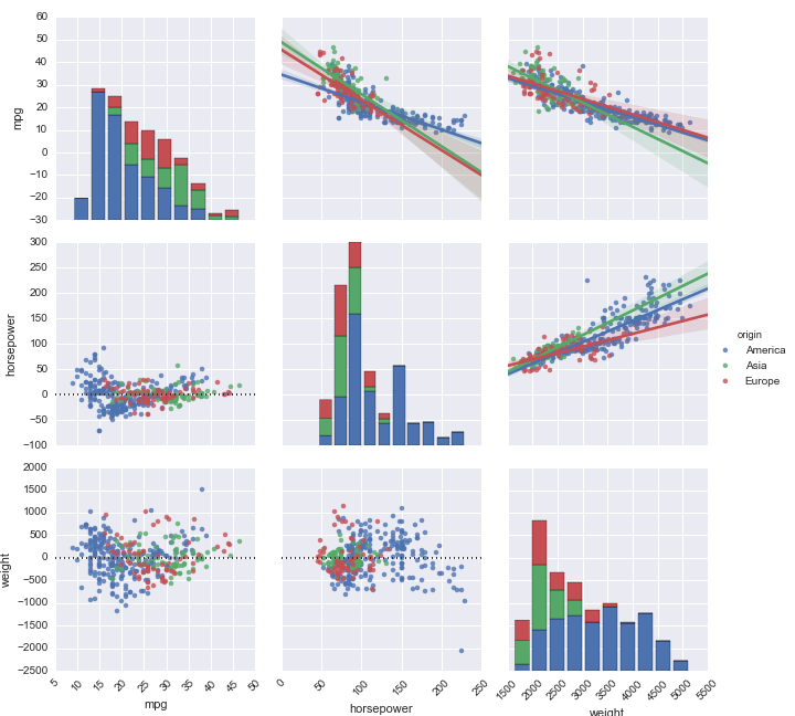
sns.set_style('darkgrid')
cols = ['SalePrice', 'OverallQual', 'GrLivArea', 'GarageCars', \
        'TotalBsmtSF', 'FullBath', 'YearBuilt']
sns.pairplot(train[cols])

At first glance, all of the predictor variables seem to have a fairly strong positive correlation with SalePrice. The only variable that's questionable is YearBuilt which looks like it could possibly have a non-linear relationship with SalePrice. Lets see:
plt.figure(figsize=(14,6))
plt.xticks(rotation=90)
sns.boxplot(x='YearBuilt', y='SalePrice', data=train)

While the relationship isn't strong, I'd say this is linear enough for a regression.
Next, I'll look at the variable that predicts SalePrice the best: Overall Quality:
plt.figure(figsize=(16,10))
sns.boxplot(x='OverallQual', y='SalePrice', data=train).set(ylabel='ln(SalePrice)')

Keep in mind that SalePrice was logarithmically transformed, but all of the values look good to test on. Next I'll handle the missing values I found in my early data exploration.
cols = ['SalePrice', 'OverallQual', 'GrLivArea', 'GarageCars', \
        'TotalBsmtSF', 'FullBath', 'YearBuilt']
sns.pairplot(train[cols])
It looks like GrLivArea and TotalBsmtSF have major outliers to the data. Lets look at those:
sns.regplot(x='GrLivArea',y='SalePrice',data=train,fit_reg=False)

#see outliers
train.sort_values(by = 'GrLivArea', ascending = False)[:2]
#drop outliers
train = train.drop(train[train['Id'] == 1299].index)
train = train.drop(train[train['Id'] == 524].index)
sns.regplot(x='GrLivArea',y='SalePrice',data=train,fit_reg=False)

sns.regplot(x='TotalBsmtSF',y='SalePrice',data=train,fit_reg=False)

It looks like TotalBsmtSF had the same outlier
test = pd.read_csv('test.csv')
test.head()
#store SalePrice for later use in model
saleprices = train['SalePrice']
data = pd.concat((train, test)).reset_index(drop=True)
data.drop(['SalePrice'], axis=1, inplace=True)
data.tail()
missing = data.isnull().sum().sort_values(ascending=False)
pct = (data.isnull().sum()/data.isnull().count()*100).sort_values(ascending=False)
#creates dataframe with missing and pct missing
miss_data = pd.concat([missing, pct], axis=1, keys=['Missing','Percent'])
#shows columns with missing values
miss_data[miss_data['Missing']>0]
As a rule, any data with more than 15% missing data is prone to messing up the data and hard to impute, so I'll drop these.
data = data.drop((miss_data[miss_data['Percent']>15]).index,1)
Garage missing values
#categorical variables
for col in ('GarageType', 'GarageFinish', 'GarageQual', 'GarageCond'):
    train[col] = train[col].fillna('NA')
#quantitative variable
train['GarageYrBlt'] = train['GarageYrBlt'].fillna(train['GarageYrBlt'].median())
Basement missing values
#categorical variables
for col in ('BsmtQual', 'BsmtCond', 'BsmtExposure', 'BsmtFinType1', 'BsmtFinType2'):
    train[col] = train[col].fillna('NA')
#quantitative variables
for col in ('BsmtFinSF1','BsmtFinSF2','BsmtUnfSF','BsmtFullBath','BsmtHalfBath'):
    test[col] = test[col].fillna(test[col].median())
Masonry Veneer missing values
#categorical variable
data["MasVnrType"] = data["MasVnrType"].fillna('NA')
#quantitative variable
data["MasVnrArea"] = data["MasVnrArea"].fillna(0)
Other missing values
Since these variables are all 'object' type with 4 or less missing values, I'll just use a filler as these missing values aren't too significant to my results
for col in ('SaleType','KitchenQual', 'Functional','MasVnrType','Exterior1st','Exterior2nd','MSZoning','Utilities','Electrical'):
    test[col] = test[col].fillna('NA')
Part 3: Feature Engineering
This part was more of a creative process. From intuition, I figured that house prices are largely affected by square footage, location, and amenities. Since location and amenities are given, I created an overall square footage feature
data['TotalSF'] = data['TotalBsmtSF'] + data['1stFlrSF'] + \
                   data['2ndFlrSF'] + data['GarageArea']
Part 4: Correcting Skewed Features
quant_feats = data.dtypes[data.dtypes != 'object'].index
skewed_feats = data[quant_feats].apply(lambda x: skew(x.dropna())).sort_values(ascending=False)
skewness = pd.DataFrame({'Skew':skewed_feats})
skewness
To fix skewness, I'll use a Box-Cox Transformation. This method tests an exponent, λ, for integers -5 to 5 and selects the λ that gives the most normal distribution using the formula:
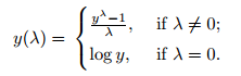 Here's a quick read on the technique: https://www.statisticshowto.datasciencecentral.com/box-cox-transformation/
from scipy.special import boxcox1p
#finds skewed features with skew greater than 1
skewness = skewness[abs(skewness)>1]
skewed_feats = skewness.index
for feat in skewed_feats:
    data[feat] = boxcox1p(data[feat],.15)
Replace Categorical Variables
data = pd.get_dummies(data)
data.head()
#uses length of train as index to split data
train = data[:train.shape[0]]
test = data[train.shape[0]:]
train.head()
I used XGBoost, which is the leading library for gradient boosting in Python. It works very similar to scikit-learn where you fit the model and run predictions
from xgboost import XGBRegressor
xgbmodel = XGBRegressor()
xgbmodel.fit(train, saleprices)
Predictions
y_pred = xgbmodel.predict(test)
y_pred
y_pred_exp = np.expm1(y_pred)
y_pred_exp
Part 6: Submission
test = pd.read_csv('test.csv')
submission = pd.DataFrame({
    'Id' : test['Id'],
    'SalePrice': y_pred_exp
})
submission.to_csv('submission.csv',index=False)
submission.head()
example = pd.read_csv('sample_submission.csv')
example.head()
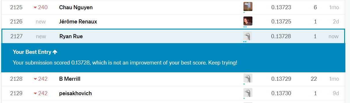
Results
Conclusion
The first time working through this journal, I did my cleaning separately on my train and test sets, but this didn't work because I got a different number of dummy variables for each due to different columns having missing values.
I also could have done more with feature engineering and created more features. Lastly, I also used XGBoost for my model, but there are thousands of different types of models, as well as ensembling methods.
Well, there we go. I went from zero to a final submission on Kaggle. I hope you enjoyed my thought process, and I'm always welcome to any comments, questions, and suggestions.