- Wed 12 September 2018
- datascience
- #logistic regression, #machine learning, #titanic
Today, I tackle the famous Titanic dataset for my first Kaggle competition.
Kaggle Machine Learning Competition: Predicting Titanic Survivors
https://www.kaggle.com/c/titanic

Competition Description
The sinking of the RMS Titanic is one of the most infamous shipwrecks in history. On April 15, 1912, during her maiden voyage, the Titanic sank after colliding with an iceberg, killing 1502 out of 2224 passengers and crew. This sensational tragedy shocked the international community and led to better safety regulations for ships.
One of the reasons that the shipwreck led to such loss of life was that there were not enough lifeboats for the passengers and crew. Although there was some element of luck involved in surviving the sinking, some groups of people were more likely to survive than others, such as women, children, and the upper-class.
In this challenge, we ask you to complete the analysis of what sorts of people were likely to survive. In particular, we ask you to apply the tools of machine learning to predict which passengers survived the tragedy.
About the Data
The data is split up into a training set and a test set.
The training set is used to build my machine learning models. For the training set, I am provided the outcome (or "ground truth") for each passenger.
The test set is used to see how well my model performs on unseen data. The ground truth is not provided, so it is my job to predict these outcomes.
There' also gender_submission.csv, a set of predictions that assume all and only female passengers survive, as an example of what a submission file should look like.
Data Dictionary
| Variable | Definition | Key |
|---|---|---|
| survival | Survival | 0 = No, 1 = Yes |
| pclass | Ticket class | 1 = 1st, 2 = 2nd, 3 = 3rd |
| sex | ex | |
| Age | Age in years | |
| sibsp | # of siblings / spouses aboard the Titanic | |
| parch | # of parents / children aboard the Titanic | |
| ticket | Ticket Number | |
| fare | Passenger fare | |
| cabin | Cabin Number | |
| embarked | Port of Embarkation | C = Cherbourg, Q = Queenstown, S = Southhampton |
Variable Notes
pclass: A proxy for socio-economic status (SES) 1st = Upper. 2nd = Middle. 3rd = Lower.
age: Age is fractional if less than 1. If the age is estimated, is it in the form of xx.5
sibsp: The dataset defines family relations in this way... Sibling = brother, sister, stepbrother, stepsister. Spouse = husband, wife (mistresses and fiancés were ignored)
parch: The dataset defines family relations in this way... Parent = mother, father. Child = daughter, son, stepdaughter, stepson. Some children travelled only with a nanny, therefore parch=0 for them.
Alright, that's all the info we need. Lets get started.
Setup Imports
import pandas as pd
import numpy as np
import matplotlib.pyplot as plt
import seaborn as sns
%matplotlib inline

import warnings
warnings.filterwarnings("ignore")
Data Exploration
Read in training data:
train = pd.read_csv('train.csv')
train.tail()
train.info()
I have 5 'object' types in my data. Later on I turn those into dummy variables so that my algorithm works.
There is also a good amount of data missing in 'Age', a ton missing in 'Cabin', and 2 missing in 'Embarked'.
train.describe()
Data Visualization
sns.set_style('darkgrid')
sns.countplot(train['Survived'])

Most people did not survive. I'll dive into each feature to see who was more likely to survive:
Feature: Passenger Class
sns.countplot(x='Survived',hue='Pclass',data=train)

Passenger class is pretty significant to if a passenger survived or not. Those in third class had a very low chance for survival in comparison to first and second class.
Feature: Sex
sns.countplot(x='Survived',hue='Sex',data=train)

Sex also seems to be a very important factor for survival. Females were very likely to live while males did not fare too well.
Feature: Age
train['Age'].hist(bins=40,edgecolor='black')

We saw earlier that the mean age was around 30 in output 6. This graph shows that the bulk of people are aged between 20-40 with a small cohort of children aged 0-16 on board.
Feature: Siblings/Spouses
sns.countplot(train['SibSp'])

Most people don't have siblings or spouses on board, with a small percent having one spouse and only a tiny percent having more than 1 spouse.
Feature: Parents/Children
sns.countplot(train['Parch'])

Again, most people don't have many spouses on board, with a small chunk with 1 or 2 parents/children.
Feature: Fare
train['Fare'].hist(bins=40,figsize=(12,4),edgecolor='black')

Most people paid very little, which makes sense because the majority of people were in third class.
Feature: Cabin
We saw earlier that there appeared to be a lot of cabin missing. Lets visualize this:
sns.heatmap(train.isnull(),yticklabels=False,cbar=False,cmap='plasma')

'Cabin' seems pretty unsavable, so I'll just remove this feature.
train.drop('Cabin',axis=1,inplace=True)
Feature: Embarked
sns.countplot(train['Embarked'])

Most passengers embarked from Southhampton, so it should be safe to fill in the 2 empty values with 'S'.
Data Cleaning
I removed the 'Cabin' feature earlier. Here I only need to fill the 'Age' and 'Embarked' columns. I'll fill in the 2 empty embarked columns with 'S', but more exploration needs to be done on age.
train['Embarked'] = train['Embarked'].fillna('S')
plt.figure(figsize=(12, 6))
sns.boxplot(x='Pclass',y='Age',data=train)

As I suspected, higher classes have a higher average age. This makes sense, because older individuals are more likely to accumulate wealth and afford a better ticket.
To fill in 'Age', I'll write a function that fills in the average age based on passenger class where 'Age' is empty. I'll then use panda's apply feature to apply this function to the 'Age' column.
def fill_age(cols):
    #define columns for use in lambda expression
    Age = cols[0]
    Pclass = cols[1]

    #returns average age for respective class if cell is empty
    if pd.isnull(Age):
        if Pclass == 1:
            return train[train['Pclass']==1]['Age'].mean()

        elif Pclass == 2:
            return train[train['Pclass']==2]['Age'].mean()

        else:
            return train[train['Pclass']==3]['Age'].mean()

    else:
        return Age
train['Age'] = train[['Age','Pclass']].apply(fill_age,axis=1)
Replace Categorical Variables
train.head(2)
train.dtypes[train.dtypes.map(lambda x: x == 'object')]
I'll get rid of 'PassengerId' since it is just another index. 'Name' and 'Ticket' are also not useful data. I will remove those variables and provide dummy variables for 'Sex' and 'Embarked'.
dum_sex = pd.get_dummies(train['Sex'],drop_first=True)
dum_embarked = pd.get_dummies(train['Embarked'],drop_first=True)
train.drop(['PassengerId','Name','Sex','Ticket','Embarked'],axis=1,inplace=True)
Now I combine my dummy variables with my updated dataframe.
train = pd.concat([train,dum_sex,dum_embarked],axis=1)
train.head()
Create Machine Learning Model
I was torn over which model to use, but I ended up chosing logistic regression for a few reasons.
Logistic regression is a simple algorithm and the go-to method for binary classification. This model translates a linear regression into a form usable for binary classification called the sigmoid function:

.gif)
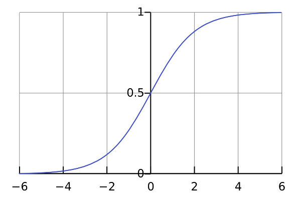
Essentially, if a p (survival in this case) is .5 or greater, it is given a value of 1. If it is a value below .5, it is assigned a value of 0. Thus, binary classification occurs.
from sklearn.linear_model import LogisticRegression
fit training data to logistic regression model:
logmodel = LogisticRegression()
logmodel.fit(train.drop('Survived',axis=1),
             train['Survived'])
Bring in test data:
test = pd.read_csv('test.csv')
test.tail()
sns.heatmap(test.isnull(),yticklabels=False,cbar=False,cmap='plasma')

The test data has all of the 'Embarked' column, but is missing a fare value! I'll have to find this value and replace it appropriately.
test[test['Fare'].isnull()]
The missing value is third class, so I'll take the average of that class and impute the missing value.
test['Fare'][152] = test[test['Pclass']==3]['Fare'].mean()
test['Fare'][152]
- apply fill_age lambda expression to fill in 'Age'
- get dummy variables for categorical variables
- create new data frame with these new values
test['Age'] = test[['Age','Pclass']].apply(fill_age,axis=1)
dum_sex = pd.get_dummies(test['Sex'],drop_first=True)
dum_embarked = pd.get_dummies(test['Embarked'],drop_first=True)
test.drop(['Name','Sex','Ticket','Cabin','Embarked'],axis=1,inplace=True)
test = pd.concat([test,dum_sex,dum_embarked],axis=1)
test.head()
I now have my data set up to run predictions on my test data!
y_pred = logmodel.predict(test.drop('PassengerId',axis=1))
y_pred
Create Submission File
submission = pd.DataFrame({
        'PassengerId': test['PassengerId'],
        'Survived': y_pred
    })
submission.to_csv('titanic.csv', index=False)
submission.head()
Compare with the given example submission called 'gender_submission':
example = pd.read_csv('gender_submission.csv')
example.head()
The submission looks good! Lets submit it and see how I did:
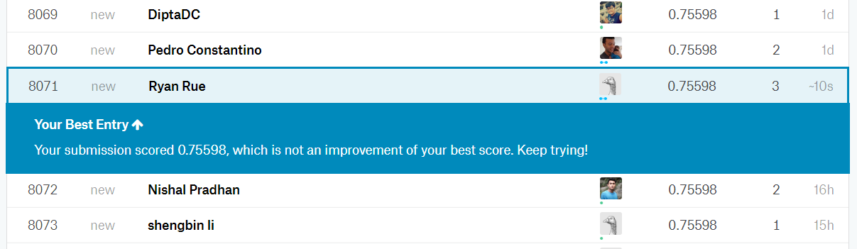
75.598% prediction rate. Not bad, though there's still lots of work that needs to be done. I think I can improve my prediction accuracy through feature engineering (maybe a column for if someone is a child), gradient boosting, or using a different machine learning model.
I hope you enjoyed this post! I'd love to hear any comments, questions, or suggestions down below. Until next time!